
Many of the functions that are used to smooth a time series tend to have a problem with lag. Here the smoothed values lag the actual values. This can cause problems for models that follow the smoothed time series. Some people have suggested the Kalman filter as a way to smooth time series without lag.
The Kalman filter has been applied to weapons targeting for radar aimed weapons. If there is significant lag in the target tracking then the target might be missed. So on this basis I thought that the Kalman filter might be good to investigate.
Unfortunately, I have had a hard time understanding the literature I've been able to find on the Kalman filter. After I completed a graduate level class on Advanced Statistics, where we covered Least Squares in great depth, I thought that I'd have another run at the Kalman filter (I read somewhere that the Kalman filter evolved from Least Squares). Unfortunately, my new knowledge was still not that helpful in understanding the material on the Kalman filter.
One of the great things about R is that you don't always have to understand how the R function is implemented. For example, the fact that a Least Squares function might be implemented with QR decomposition does concern the user of the R lm() function.
As it turns out, however, the R documentation for the Kalman filter is not terribly easy to understand either. However, I was able to write some R code to do the Kalman filter.
The model that I have for smoothing is for a dynamic time series. Some number of initial values have been collected. The filter is applied and the last value in the smoothed data set is used as the first value in the smoothed time series. Then another value is added and the data is smoothed again, producing another smoothed point.
This means that the Kalman filter code is run for every smoothed point. The Kalman filter is fairly compute intensive, so this makes the code very slow. It could not, for example, be used for intraday "tick" data, since its too slow.
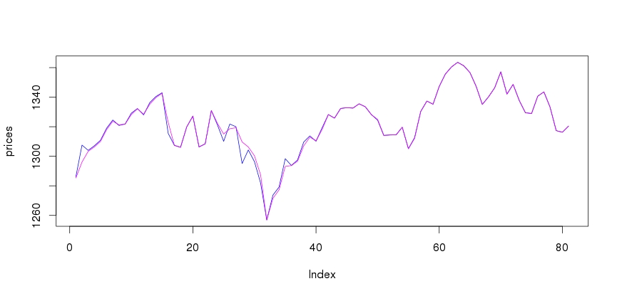
This code does provide some idea of how the Kalman filter works for smoothing. The blue line in the plot is the original time series. The magenta line is the smoothed time series.
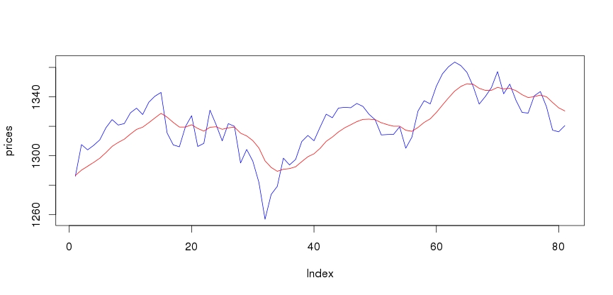
By way of comparison, the plot below shows an exponential moving average smooth (EMA) with a window of 20.
library(KFAS)
library(tseries)
library(timeSeries)
library(zoo)
library(quantmod)

getDailyPrices = function( tickerSym, startDate, endDate )
{
  prices = get.hist.quote( instrument = tickerSym, start = startDate, end = endDate,
                       quote="AdjClose", provider="yahoo",
                       compression="d",  quiet=T)

  prices.ts = ts(prices)
  return( prices.ts )
}

kalmanFilter = function( x )
{
  t = x
  if (class(t) != "ts") {
    t = ts(t)
  }
  ssModel = structSSM( y = t, distribution="Gaussian")
  ssFit = fitSSM(inits=c(0.5*log(var(t)), 0.5*log(var(t))), model = ssModel )
  kfs = KFS( ssFit$model, smoothing="state", nsim=length(t))
  vals = kfs$a
  lastVal = vals[ length(vals)]
  return(lastVal)
}

Start = "2011-01-01"
End   = "2012-12-31"
SandP = "^GSPC"

windowWidth = 20
tsLength = 100

SAndP.ts = getDailyPrices( SandP, Start, End )
SAndP.ts = SAndP.ts[1:tsLength]
SAndP.smoothed = rollapply( data=SAndP.ts, width=windowWidth, FUN=kalmanFilter)

par(mfrow=c(1,1))
prices = coredata( SAndP.ts[windowWidth:length(SAndP.ts)])
plot(prices, col="blue", type="l")
lines(coredata(SAndP.smoothed), col="magenta")
par(mfrow=c(1,1))
|
The code for the EMA filter is shown below:
library(TTR)

emaSmooth = function( x )
{
  ema = EMA(x)
  val = ema[ length(ema) ]
  return(val)
}

emaSmooth = rollapply( data = SAndP.ts, width=windowWidth, FUN=emaSmooth)
|
The limitations in my understanding of the Kalman filter may have resulted in misuse here. On thing that I noticed in experimenting with this code is that as the window gets larger, the filter gets closer to the time series and there is less smoothing. This is not what I would have naively expected.
Ian Kaplan
January, 2013