Notes on a simple industry factor model

These notes are heavily based on Chapter 15 of Modeling Financial Time Series with S-Plus by Zivot and Wang, Second Edition, Springer, 2006. In places I have taken the liberty of copying complete sentences (or parts of sentences). Other material has been cribbed from Prof. Zivot's lecture notes for his Factor Models for Asset Returns lecture.

The S+ code in Zivot and Wang can be used almost without change in R. A few of the necessary changes have been taken from the code that Guy Yollen used in Financial Data Modeling and Analysis with R (AMATH 542), which is part of the University of Washington Computational Finance Master's program.

These notes are not intended to be an original work. They are not a paper or an article. So I hope that Prof. Zivot and Wang will not object to my borrowing their material. Any errors, however, are mine.

Least Squares Linear Regression

Factor models are linear models: where are the predictor variables and is the response variable. Linear regression is used to estimate the values. The vectors are If there is a matrix, X, then the linear model can be written as , where the values are estimated via least squares. The least squares equation to estimate is .

Fundamental Factor Models

BARRA style single factor model:

The values are known and are invariant (at least over the time period t = 1...T). The factor value, is estimated from the data. An example of such a value would be industry sector and industry membership for a stock. Here each stock, i = 1...N, has its asset specific value of .

The expression for a mutli-factor model is:

where is the return (real or in excess of the risk free rate) on asset i (i = 1..N) in time period t (t = 1..T). This is a linear factor model, where is the intercept, is the common factor (k = 1..K), is the factor loading or factor beta for asset i on the factor, and is the asset specific factor.

The return on asset 1, at time t1 is

Cross Sectional Models

A cross sectional view of the factor model is shown in the equation below. Here the cross section is across a single unit of time, t1. Here the cross sectional return for all of the assets (I = 1..N) is calculated at time t1.

This can be rewritten incorporating the intercept term (the values) into the beta matrix:

In the fundamental factor model, the beta values (B) are known and the factor values () are unknown.

The ordinary least squares equation for (for multiple linear regression) is: where the B values are invariant (for example, industry membership) and the values are the returns. To calculate the cross sectional regression we calculate the factor realizations

BARRA Factor models

In portfolio construction factor models are used to estimate the covariance matrix, , that is used to estimate the optimal portfolio (either the mean-variance or CVaR optimal portfolio).

The beta values, (for asset i and industry k) are 1 if asset i is in industry k, and zero otherwise.

The factor values, (for industry k at time t, t = 1...T) are equal to the weighted excess return for the firms in the portfolio that are in industry k.

To estimate the weighted least squares we first need to find the error variance. This is found via ordinary least squares of the result of the cross sectional regression, at time t.

The BARRA style industry factors are stored in the matrix B (here we can assume that the matrix has the column and row names shown below):

There is also a matrix of returns for fifteen stocks listed above. To estimate :

F.hat = solve(t(B) %*% B) %*% t(B) %*% t(returns)

Calculate the residual variances and build the matrix. The matrix is a diagonal matrix containing the values.

In least the least squares equation above, the residual variance is . Here the residual variance is

E.hat = t(returns) - B %*% F.hat

Calculate the variances across the rows

diagD.hat = apply(E.hat, 1, var)

Dinv.hat = diag( diagD.hat^(-1))

Note that the inverse of the matrix D is the same as the inverse of the values on the diagonal:

identical(solve(diag(diagD.hat)), diag(diagD.hat^(-1))) is TRUE

# multivariate FGLS regression to estimate K x T matrix of factor returns

H = solve(t(B) %*% Dinv.hat %*% B) %*% t(B) %*% Dinv.hat

# create factor mimicking portfolios

F.hat = H %*% t(returns)

colnames(H) = colnames(returns)

F.hat = t(F.hat)

The rows of the H matrix contain the weights for the factor mimicking portfolio:

Estimation of Industry Factor Model Asset Return Covariance Matrix. The covariance matrix of the N assets is then estimated by:

cov.ind = B %*% var(F.hat) %*% t(B) + diag(diagD.hat)

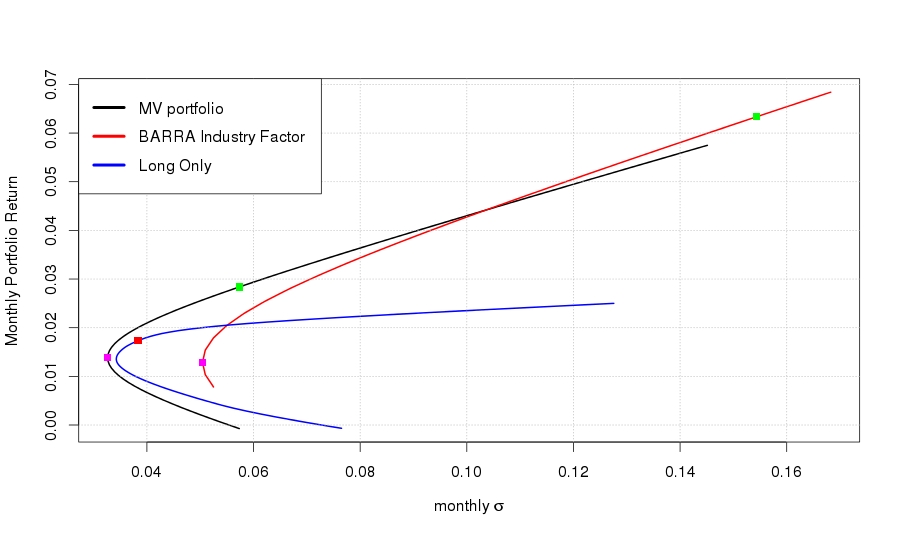
The plot below shows efficient frontiers for a mean-variance optimized long/short portfolio, the BARRA industry factor model, developed above and a mean-variance long only portfolio.

A listing of the complete R code can be found here.

The R code and the model data can be downloaded here:

1. berndtInvest.csv (this data was originally from the R fEcofin package, from Rmetrics. At the time of this writing, this package had become unavailable.
2. industry_factor.r

Fama-French Factor Model

The Fama-French approach for estimating for a given characteristic (for example market capitalization size) they use a two step process:

1. Sort the cross section of assets based on the values of the asset specific characteristics.

2. Form a hedged portfolio that is long in the top quintile (e.g., top 20%) for the characteristic and short in the bottom quintile of the sorted assets. This portfolio is a dollar neutral portfolio (e.g., as much on the long side as the short side).

The return on the hedged portfolio at time t is the observed factor realization for the asset specific characteristic . The process is repeated for each factor, over the time period t = 1..T.

This gives us a set of cross sectional values for each factor i, i = 1...N. The factor values are estimated using N time series regressions.

Time Series Model

The factor model can also be expressed as a time series model, where the return on asset is calculated across the time period t = 1...T.

For BARRA style fundamental factor models, the values are constant and the factor realizations at time t, are estimated from the data.

This can be written as the ordinary least squares equation

back to Topics in Quantitative Finance